Introduction to DAX
Data Analysis Expressions (DAX) is a programming language that is used throughout Microsoft Power BI for creating calculated columns, measures, and custom tables. It is a collection of functions, operators, and constants that can be used in a formula, or expression, to calculate and return one or more values. You can use DAX to solve a number of calculation and data analysis problems, which can help you create new information from data that is already in your model.
In Power BI, you can use different calculation techniques and functions to create measures or calculated columns. Primarily, you will be able to achieve the same result by using these techniques; however, the key is to know how and when to apply them. By having a basic understanding of when and how to use which technique, you will be able to create robust and high-performance data models.
Use calculated columns
DAX allows you to augment the data that you bring in from different data sources by creating a calculated column that didn't originally exist in the data source. This feature should be used sparingly, which will be explained later in this module.
For example, assume that you are importing data from a database that contains sales transactions. Each individual sales transaction has the following columns: Order ID, Product ID, Quantity, and Unit Price. Notice that a column doesn't exist for the total sales amount for each order.
The following figure shows how the initial shape of the data appears in a Power BI table visual.
You can start using DAX by creating a calculated column that multiplies the unit price with the quantity. The calculated column will create a value for each row called Total Price. Create the new column by selecting the ellipsis (...) button on the table in the Fields list and then selecting New column.
A new DAX formula appears in the formula bar underneath the ribbon at the top.
You can replace the "Column =" default text with the following example text:
Total Price = 'Sales OrderDetails'[Quantity] * 'Sales OrderDetails'[Unit Price]
The value on the left side of the equal sign is the column name. The text on the right side of the equal sign is the DAX expression. This simple DAX expression takes the quantity value and multiplies it with the unit price value for each individual row. It will produce one value for each record in the table. If you drag the new column from the Fields list to the visual, you will see the new values.
The previous screenshot shows that DAX is calculating correctly and displaying the results that you wanted.
Calculated columns are materialized in the .pbix Power BI file extension, meaning that each time you add a calculated column, you are increasing the size of the overall file. Having too many calculated columns will slow performance and will cause you to reach the maximum Power BI file size sooner.
Create a custom column
Three ways to create a custom column in Power BI are:
Create the column in the source query when you get the data, for instance, by adding the calculation to a view in a relational database.
Create a custom column in Power Query.
Create a calculated column by using DAX in Power BI.
You can create a calculated column when you pull the data from the data source. Each data source would have a different technique for completing this action. For instance, if you were pulling data from a relational data source by using a view that was written in the SQL language, it would look like the following example:
CREATE VIEW OrdersWithTotalPrice
AS
SELECT unitprice, qty, unitprice * qty as TotalPrice
FROM sales.salesorders
Using SQL language is an efficient way of creating a column because it would make the data source do the calculations for you. In Power BI, the calculated column would appear like any other column.
You can also use Power Query to create a custom column.
The custom column dialog uses the M language to create the new column. M language is out of scope for the purposes of this module.
The third way to create a calculated column is by using DAX in Power BI, as previously demonstrated.
When you create a calculated column by using DAX, you do not need to refresh the dataset to see the new column. In the other methods, you would need a refresh to see changes. This process can be lengthy if you are working with a lot of data. However, this issue is irrelevant because, after columns have been created, they are rarely changed.
The DAX calculated column does not compress as well as the other methods. The other column types do get compressed, which makes the .pbix file smaller and the performance usually faster.
Generally, the earlier you can create a column, the better. It is not considered an optimal practice to use DAX for calculations if you can use a different mechanism.
In addition, one way to avoid using a calculated column is to use one of the X functions, such as SUMX, COUNTX, MINX, and so on. The X functions are beyond the scope of this module; however, they allow you to create measures that are aware of the data in individual rows and calculate totals based on the totals in the row. These functions are called iterator functions because, though they are used in measures, they iterate over the individual rows to do their calculations. An X function will perform better and use less disk space than a calculated column. For more information about X functions, see the Microsoft documentation.
Use measures
Calculated columns are useful, when you are required to operate row by row. However, other situations might require a simpler method. For example, consider a situation where you want an aggregation that operates over the entire dataset and you want the total sales of all rows. Furthermore, you want to slice and dice that data by other criteria like total sales by year, by employee, or by product.
To accomplish those tasks, you would use a measure. You can build a measure without writing DAX code; Power BI will write it for you when you create a quick measure.
Many available categories of calculations and ways to modify each calculation exist to fit your needs. Another advantage is that you can see the DAX that's implemented by the quick measure while jumpstarting or expanding your own DAX knowledge.
Create a quick measure
To create a quick measure in Power BI Desktop, right-click or select the ellipsis (...) button next to any item in the Fields pane and then select New quick measure from the menu that appears. The Quick measures screen will appear.
In the Quick measures window, you can select the calculation that you want and the fields to run the calculation against. For instance, you can select a calculation and the column that you want to operate over. Power BI creates the DAX measure for you and displays the DAX. This approach can be a helpful way to learn the DAX syntax.
Create a measure
Measures are used in some of the most common data analyses.
To continue with the previous scenario, you want to create a measure that totals your new column for the entire dataset. Similar to how you created a calculated column, you can go to the Fields list, click the three-dot ellipsis on the selected field and select New measure.
Text will now appear in the formula bar underneath the ribbon.
You can replace the "Measure =" text with the following text:
Total Sales = sum('Sales OrderDetails'[Total Price])
The new measure will now appear in the Fields list.
When you drag Total Sales over to the report design surface, you will see the total sales for the entire organization in a column chart.
Differences between a calculated column and a measure
The fundamental difference between a calculated column and a measure is that a calculated column creates a value for each row in a table. For example, if the table has 1,000 rows, it will have 1,000 values in the calculated column. Calculated column values are stored in the Power BI .pbix file. Each calculated column will increase the space that is used in that file and potentially increase the refresh time.
Measures are calculated on demand. Power BI calculates the correct value when the user requests it. When you previously dragged the Total Sales measure onto the report, Power BI calculated the correct total and displayed the visual. Measures do not add to the overall disk space of the Power BI .pbix file.
Measures are calculated based on the filters that are used by the report user. These filters combine to create the filter context.
Understand context
How context affects DAX measures is a difficult concept to comprehend. The ensuing visuals will demonstrate how context affects DAX measures so you can see how they interact together.
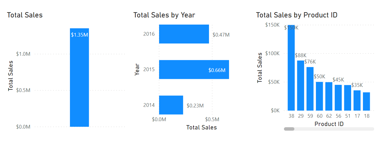
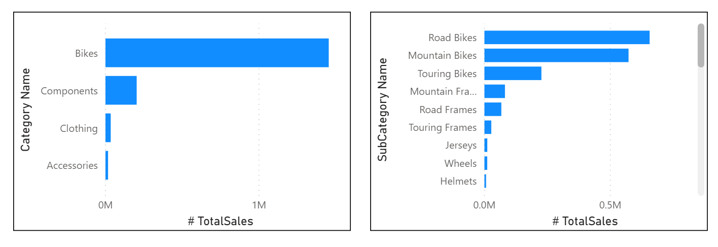
The following three visuals use the exact same DAX measure: Total Sales.
Though each visual uses the same DAX measure and, therefore, the same DAX formula, the visuals produce different results. For instance, the first visual shows the Total Sales measure for the entire dataset. In this dataset, Total Sales is USD1.35 million. In the second visual, Total Sales is broken down by year. For instance, in 2014, Total Sales is USD0.23 million. In the third visual, Total Sales is broken down by Product ID.
With Power BI, even though the measure was only defined once, it can be used in these visuals in different ways. Each of the totals is accurate and performs quickly. It is the context of how the DAX measure is used that calculates these totals accurately.
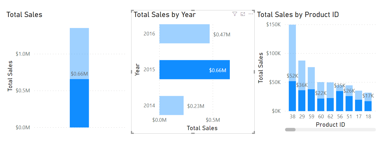
Interactions between visuals will also change how the DAX measure is calculated. For instance, if you select the second visual and then select 2015, the results appear as shown in the following screenshot.
Selecting 2015 in the second visual changed the filter context for the DAX measure. It modified the first visual to equal the sales for 2015: USD0.66 million. It also broke down the Total Sales By Product ID, but only shows the results for 2015. Those calculations quickly changed in memory and displayed the results in a highly interactive manner to the user.
The definition of the DAX measure has not changed; it's still the original, as shown in the following example:
Total Sales = sum('Sales OrderDetails'[Total Price])
This scenario is a simple way to explain how context works with DAX. Many other factors affect how DAX formulas are evaluated. Slicers, page filters, and more can affect how a DAX formula is calculated and displayed.
Use the Calculate function
The CALCULATE function in DAX is one of the most important functions that a data analyst can learn. The function name does not adequately describe all it is intended to do.
The CALCULATE function is your method of creating a DAX measure that will override certain portions of the context that are being used to express the correct result.
For instance, if you want to create a measure that always calculates the total sales for 2015, regardless of which year is selected in any other visual in Power BI, you would create a measure that looks like the following sample:
Total Sales for 2015 = CALCULATE(SUM('Sales OrderDetails'[Total Price]), YEAR('Sales OrderDetails'[orderdate]) = 2015)
Notice how the measure is named Total Sales for 2015. When you use the CALCULATE function to override the context, it is helpful to name the measure in a way that describes exactly how you are overriding it. In this example, CALCULATE is aggregating the Total Price column, just as you did in the previous measure. However, instead of operating over the entire dataset while using whatever the filter context tells it to do, you are overriding the filter context for the year 2015. No matter what year is selected as a filter for other reports, you will always get the total for 2015 using this measure; all other filters still apply. The subsequent example shows this concept in action.
When both measures are added to the previous visual they will resemble the following screenshot.
As shown in the preceding screenshot, Total Sales is still USD1.35 million, while the 2015 Total Sales is USD0.66 million.
When you add the other visual onto the report, as you did previously, and then select 2015, the results will look like the following image. If you select 2016, Total Sales for 2015 will remain at USD0.66 million.
Notice how both measures are now equally the same amount. If you were to filter by any other criteria, including region, employee, or product, the filter context would still be applied to both measures. It's only the year filter that does not apply to that measure.
Use relationships effectively
Another DAX function that allows you to override the default behavior is USERELATIONSHIP.
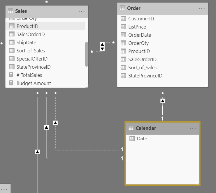
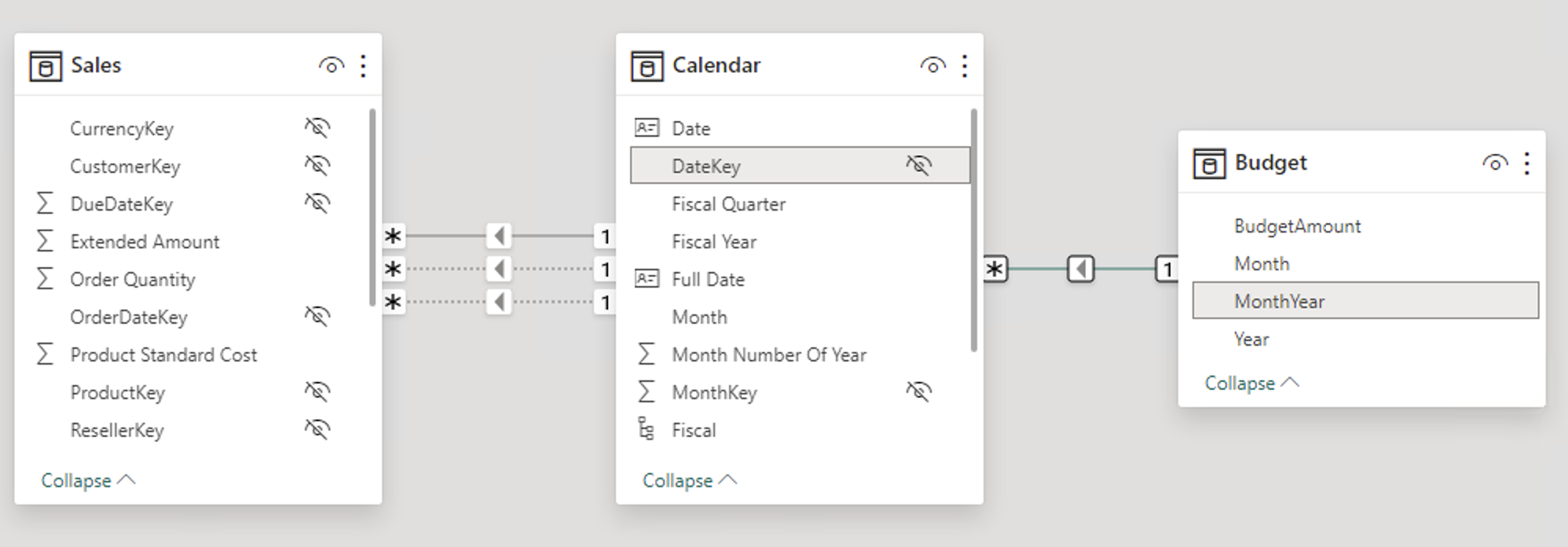
Consider the following data model example.
The preceding screenshot shows an established relationship between the Date and OrderDate columns, as shown by the highlighted line connecting the two. The solid line between the two tables indicates that it is the active relationship, meaning that by default, any slicing on the date table where measures in the Sales data are being displayed will be along the OrderDate column. A dashed relationship exists between the Date and ShipDate columns, indicating that it is an inactive relationship. This relationship will never be used unless explicitly declared in a measure.
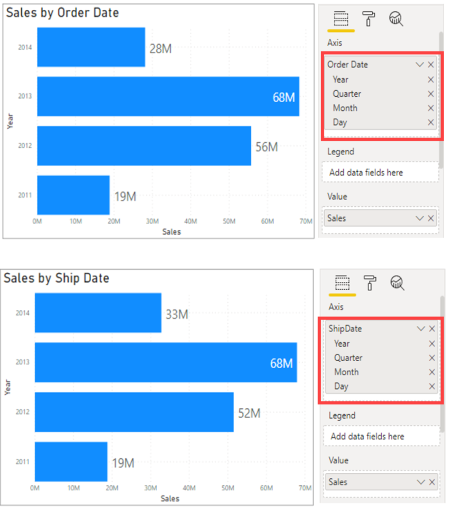
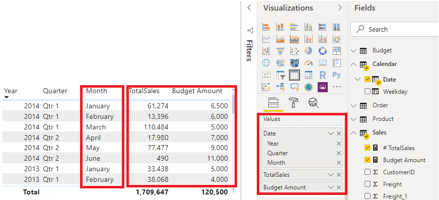
The goal is to build the following report, where you have two visuals: Sales by Ship Date and Sales by Order Date.
These visuals show the sales over time, but the first visual is by order date and the second is by ship date so, though they are both dates, a different data point is associated with them to get both sets of data on the same visual.
To create this measure for Sales by Ship Date, you can use the DAX function USERELATIONSHIP(). This function is used to specify a relationship to be used in a specific calculation and is done without overriding any existing relationships. It is a beneficial feature in that it allows developers to make additional calculations on inactive relationships by overriding the default active relationship between two tables in a DAX expression, as shown in the following example:
Sales by Ship Date = CALCULATE(Sum(Sales[TotalPrice]), USERELATIONSHIP(Sales[ShipDate],'Calendar'[Date]))
Create semi-additive measures
In situations where you don't want the standard evaluation behavior in Power BI, you can use the CALCULATE and/or USERELATIONSHIP functions. However, more circumstances exist where you don't want the standard behavior. One of those situations is when you have a semi-additive problem to resolve. Standard measures are simple concepts, where they might use the SUM, AVERAGE, MIN, and MAX functions. Thus far, you've been using SUM for the Total Sales measure.
Occasionally, summing a measure doesn't make sense, such as when you are performing inventory counts in a warehouse. For example, if on Monday, you have 100 mountain bikes, and on Tuesday you have 125 mountain bikes, you wouldn't want to add those together to indicate that you had 225 mountain bikes between those two days. In this circumstance, if you want to know your stock levels for March, you would need to tell Power BI not to add the measure but instead take the last value for the month of March and assign it to any visual.
You can use the CALCULATE function to complete this action, along with the LastDate function, as shown in the following example:
CALCULATE (
    SUM ( 'Warehouse'[Inventory Count] ),
    LASTDATE ( 'Date'[Date] ))
This approach will stop the SUM from crossing all dates. Instead, you will only use the SUM function on the last date of the time period, thus effectively creating a semi-additive measure.
Work with time intelligence
All data analysts will have to deal with time. Dates are important, so we highly recommend that you create or import a dates table. This approach will help make date and time calculations much simpler in DAX.
While some time calculations are simple to do in DAX, others are more difficult. For instance, the following screenshot shows what happens if you want to display a running total.
Notice that the totals increment for each month but then reset when the year changes. In other programming languages, this result can be fairly complicated, often involving several variables and looping through code. DAX makes this process fairly simple, as shown in the following example:
(
    SUM('Sales OrderDetails'[Total Price])
    , Dates[Date]
)
The YTD Total Sales measure uses a built-in DAX function called TOTALYTD. This function takes an argument for the type of calculation. You can use the SUM function to get the Total Price, as you've done throughout this module. The second argument that you want to operate over is the Dates field. You can use your Dates table and add this measure to your visual, and you'll get the running total result that you're looking for. You can use all functions with YTD, MTD, and QTD in a similar fashion.
Another example of working with time would be comparing your current sales with the sales of a previous time period. For instance, if you want to see the total sales of the month next to the total sales of the prior month, you would enter the DAX measure definition, as shown in the following example:
Total Sales Previous Month = CALCULATE
(
    sum('Sales OrderDetails'[Total Price])
    , PREVIOUSMONTH(Dates[Date])
)
This measure uses the CALCULATE function, indicating that you're overriding the context to evaluate this expression the way that you want to. You're summing Total Price, as you've been doing throughout this module. For the second argument, you're using PREVIOUSMONTH for the override, which tells Power BI that, no matter what month is the default, the system should override it to be the previous month.
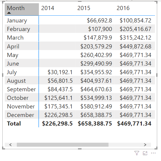
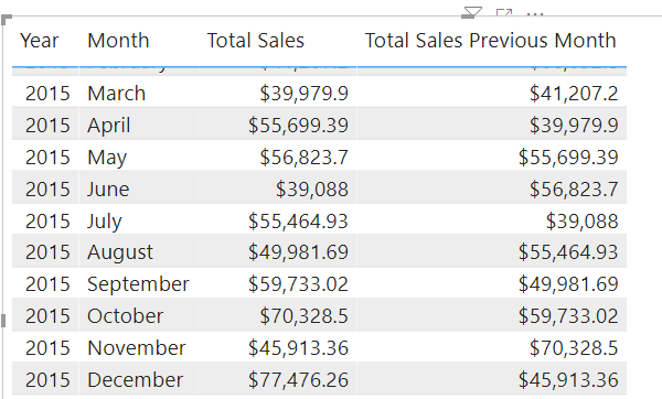
The following screenshot shows the results in a table visual.
When you examine the months side-by-side, notice that the total sales for July compare to the total sales for June.


